```{r}
2 + 2
```[1] 4Hands on
In brief, Quarto allows you to combine various types of content in a document (text, code, equations, images, graphics, etc.) and then compile it all into a single document, such as HTML, PDF, etc. The term used in the Quarto environment for this compilation is very poetically called knitting.
Today, we will explore the data from the Palmerpenguins package to answer the following questions:
What is the relationship between flipper length and body mass?
Does this relationship vary between species?
To ensure transparency and reproducibility, we will create a Quarto report.
But first, let’s get a grasp of the basics and create our first Quarto document!
.qmd) by navigating to File > New File > Quarto DocumentUse visual markdown editor” option. Finally, click Create.qmd file on you computer (preferably in an appropriate folder)Render to render/knit your document. Observe the result. What type of document is this?docx)pdf)?The most common thing you are likely to do in your Quarto document is text formatting. The language used for this is called Markdown. It is a fairly basic language but allows you to intuitively perform most basic formatting tasks.
Markdown-formatted document should be publishable as-is, as plain text, without looking like it’s been marked up with tags or formatting instructions. - John Gruber
Formatting text is easy and often follows a common structure by surrounding the text you want to format with special characters:
*italic* **bold** ~~strikeout~~ `code`

superscript^2^ subscript~2~

[underline]{.underline} [small caps]{.smallcaps}
italic bold
strikeoutcodesuperscript2 subscript2
underline small caps
Sections are added to a document using different numbers of #:
# 1st Level Header

## 2nd Level Header

### 3rd Level Header- Bulleted list item 1
- Item 2
- Item 2a
- Item 2b
1. Numbered list item 1
2. Item 2
i) Sub-item 1
A. Sub-sub-item 1
Bulleted list item 1
Item 2
Item 2a
Item 2b
Numbered list item 1
Item 2
sub-item 1
A. sub-sub-item 1
Markdown is case-sensitive in some cases, meaning you need to format the text correctly for it to recognise a sub-item, for example. For lists, you often need to add a space before and after.
Add a link with angle brackets for displaying the raw URL, or use a combination of square and round brackets to define the link text and URL:
<https://quarto.org/>

A link to the [Quarto documentation](https://quarto.org/).A link to the Quarto documentation.
Add an image using .
You can add a caption easily within the brackets as such: 

Use relative file paths rather than absolute file paths - other people won’t share the same absolute file path as you!
File paths are relative to where the Quarto document is!
Download the penguins-template.qmd zip
Unzip the downloaded folder and, if you want, rename the unzipped folder on your computer (something like “cs-workshop-2025”)
Now, open the penguins-template.qmd file in Rstudio
Once Rstudio is up and running, copy and paste install.packages("palmerpenguins") into the Console and run it once
Add a Level 2 header titled “Data description” after the existing content in the penguins-template.qmd file. Render and observe.
Copy and paste the following text into the file:
The penguins dataframe contains 344 observations of penguins.
It includes several qualitative variables, including the following:

Sex of the penguins
Island where they are found
Species to which they belong

The represented species are: Chinstrap, Gentoo, and Adelie.
Format the text so that the final rendering looks like this:
The
penguinsdataframe contains 344 observations of penguins. It includes several qualitative variables, including the following:
- Sex of the penguins
- Island where they are found
- Species to which they belong
The represented species are : Chinstrap, Gentoo et Adelie.
Render and observe.
Add the online image found at this link to your document. What does this image represent?
Add a caption to this image.
Render your document for the last time. Observe the changes.
Code chunks are the main way of including executable code in a document. In our case, we’ll be using R.
A code chunk usually starts with ```{r} and ends with ```. You can write any number of lines of code in it.
To insert a code chunk, click Code > Insert Chunk.
```{r}
2 + 2
```
[1] 4The result is outputted after the chunk, as you can see.
A more coherent example:
```{r}
library(ggplot2)
library(palmerpenguins)
```
Warning: le package 'palmerpenguins' a été compilé avec la version R 4.4.2```{r}
data(penguins)
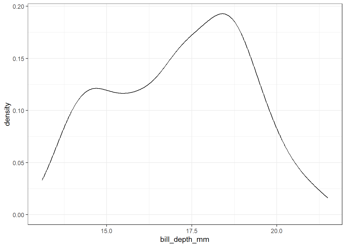
``````{r}
ggplot(data = penguins,
mapping = aes(x = bill_depth_mm)) +
geom_density() +
theme_bw()
```Warning: Removed 2 rows containing non-finite outside the scale range
(`stat_density()`).
We can change the chunk execution options so that the code messages do not show, by adding #| warning: false.
```{r}
#| warning: false

ggplot(data = penguins,
       mapping = aes(x = bill_depth_mm)) +
  geom_density() +
  theme_bw()
```
Most common execution options:
| Option | Description if ____: true |
|---|---|
eval |
Evaluate the code chunk |
echo |
Include the source code in output |
output |
Include the results of executing the code |
warning |
Include warnings/messages in the output |
error |
Include errors in the output (errors won’t halt document processing) |
include |
Prevent any output (code or results) from being included |
code-foldInstead of simply removing the code, we can choose to include code but have it hidden by default.
```{r}
#| warning: false
#| code-fold: true

ggplot(data = penguins,
       mapping = aes(x = bill_depth_mm)) +
  geom_density() +
  theme_bw()
```
fig-```{r}
#| warning: false
#| fig-align: center
#| fig-width: 4
#| fig-asp: 0.9
#| fig-cap: "Distribution of bill depth sizes"
ggplot(data = penguins,
mapping = aes(x = bill_depth_mm)) +
geom_density() +
theme_bw()
```
labelWe can add internal links for cross-referencing using label.
```{r}
#| warning: false
#| fig-align: center
#| fig-width: 4
#| fig-asp: 0.9
#| fig-cap: "Distribution of bill depth sizes"
#| label: fig-billdepth

ggplot(data = penguins,
       mapping = aes(x = bill_depth_mm)) +
  geom_density() +
  theme_bw()
```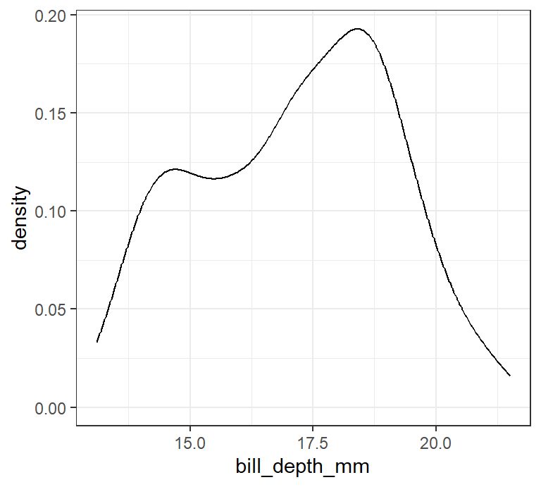
Many penguins in the dataset seem to have a bill depth between 18 and 19mm ([@fig-billdepth]).Many penguins seem to have bill depths between 18 and 19mm (Figure 1).
tbl-) and equations (eq-)Table options are similar to those of figures, but instead of fig- for some options, it is tbl-:
```{r}
#| tbl-align: center
#| tbl-cap: "First 5 rows and columns of the penguins dataset"
#| label: tbl-pengdata

knitr::kable(head(penguins[,1:5]))
```| species | island | bill_length_mm | bill_depth_mm | flipper_length_mm |
|---|---|---|---|---|
| Adelie | Torgersen | 39.1 | 18.7 | 181 |
| Adelie | Torgersen | 39.5 | 17.4 | 186 |
| Adelie | Torgersen | 40.3 | 18.0 | 195 |
| Adelie | Torgersen | NA | NA | NA |
| Adelie | Torgersen | 36.7 | 19.3 | 193 |
| Adelie | Torgersen | 39.3 | 20.6 | 190 |
For equations, it is slightly different for cross-referencing.
$$
E = mc^2
$$ {#eq-linear}
\[ E = mc^2 \tag{1}\]
According to the @eq-linear, the relationship between energy and mass is directly proportional.According to the Equation 1, the relationship between energy and mass is directly proportional.
You can include executable expressions inside the markdown (text) by enclosing the expression in `r `
Example: The penguins dataset is composed of `r nrow(penguins)` observations.
The penguins dataset is composed of 344 observations.
Add a code chunk to generate a table showing the first 5 rows of the penguins dataframe using the knitr::kable() function. Render and observe.
For those not familiar with R, unfold the following, copy and paste inside the code chunk, and render:
knitr::kable(head(penguins))Add another Level 2 header, this time titled “Data visualisation”
Add a second code chunk to generate a figure (using R base or ggplot2) to explore the relationship between the body mass of penguins and the length of their flippers, as well as the differences between species. Render and observe.
For those not familiar with R, unfold the following, copy and paste inside the code chunk, and render:
g <- ggplot(penguins, aes(x = flipper_length_mm,
                              y = body_mass_g)) +
      geom_point(aes(color = species, shape = species),
                 size = 2,
                 alpha = 0.7) +
      scale_color_manual(values = c("darkorange","purple","cyan4")) +
      labs(x = "Flipper length (mm)",
           y = "Body mass (g)",
           color = "Penguin species",
           shape = "Penguin species") +
      theme_minimal()

g
Add the following options to the code chunk, one by one. Render the document after each modification and observe the changes:
echo: false
warning: false
Just below the figure, provide a description of the relationship between the two variables, both overall and for each species.
Modify the size of the figure using the following options, one by one. Render the document after each modification and observe how the figure changes:
fig-width: 10
fig-height: 3
out-width: "100%"
out-width: "20%"
Add a label to the figure with the prefix fig-.
Add a caption to the figure using the fig-cap chunk option. In the description written in at 4., add the cross-reference to this figure. Render and observe.
Well done! You’ve just created your first Quarto report 🎉
There is so much more you can do with Quarto, such as:
And so much more…
Check out the full Quarto documentation and the resources available on this site.
Yet Another Markup Language, corresponding the the metadata of a Quarto document↩︎