Graphical abstract of the Cluefish workflow.
Preface
This vignette is intended to help users who wish to use Cluefish. The first part of this vignette is dedicated to an introduction of the context in which Cluefish was developped, followed by an overview of the workflow. The second part is dedicated to a step-by-step guide of the main Cluefish workflow using an example dose-response (DR) dataset.
Introduction
A bit of context
In transcriptomics, analyses yield extensive transcript lists that require impractical manual literature reviews. To address this, functional enrichment (FE) analysis, also known as pathway enrichment analysis, has become the standard approach. This method condenses large gene lists into more manageable and interpretable sets of biological functions or pathways (Das, McClain, and Rai 2020). FE relies on predefined gene sets representing molecular functions, biological processes or pathways, as outlined by resources like the Gene Ontology (GO) (Ashburner et al. 2000) or pathway databases such as KEGG (Kanehisa and Goto 2000) and Wikipathways (Martens et al. 2021).
FE approaches have evolved in four generations: Over-Representation Analysis (ORA), Functional Class Scoring (FCS), Pathway Topology (PT), and Network Topology (NT)-based methods1.
Each generation introduced improvements by accounting for gene co-expression, pathway topology, and network crosstalk. However, PT and NT-based approaches face limitations due to incomplete pathway and network information for lesser studied organisms, making ORA and FCS the most widely used methods (Liu, Wei, and Ruan 2017).
While these earlier methods are commonly applied to transcriptomic data with two or three conditions, dealing with data involving many ordered conditions—referred to as “data series”—poses substantial complexity.
In dose-response (DR) studies, which explore the relationship between
exposure and biological effect, DR omics analyses play a critical role
(Lovell 2016). Unlike standard
differential expression analyses, DR methods, such as the DRomics
(Dose-Response for Omics) R package (Larras et
al. 2018), model the full DR relationship of each transcript
rather than just fold-change between conditions. From these models, a
benchmark dose (BMD) is calculated for each transcript : a dose that
represents a specific change in response, indicating a gene’s
sensitivity to a stressor (Committee et al.
2017).
While differential gene expression analysis provides fold-change
values and their associated p-values, modelling approaches, such as
DRomics, characterise the entire DR relationship. PT-based
enrichment and FCS, which rely on fold-change values, are therefore not
adapted for functional enrichment in a DR context (Khatri, Sirota, and Butte 2012). ORA is
currently the only suitable method available to complement DR modelling,
as it exclusively uses deregulated gene lists. However, ORA comes with
several other limitations. The enrichment results, often based on
Fisher’s Exact Tests, can be biased towards broad biological functions,
since using all deregulated genes makes it harder to reach statistical
significance for smaller or specialised functions. This tendency is
intrinsically tied to the granularity of gene sets in certain databases
(e.g., GO). Gene sets associated to a biological process/pathway may be
overly specific, while others are too general, potentially compromising
the relevance of the analysis (Karp et al. 2021;
Mubeen et al. 2022). Additionally, gene sets may vary in
specificity, and results often reflect only part of the deregulated gene
list. Therefore, ORA alone (hereafter referred to as the
“standard approach”) is insufficient for interpreting
complex DR data, and combining additional methods is essential to
capture a fuller and more precise view of the biological context.
Overview of Cluefish
To address these limitations, we developed Cluefish (Franklin et al. (2025)), a free and open-source, semi-automated workflow designed for comprehensive and untargeted exploration of transcriptomic data series. Its name reflects the three key concepts driving the workflow: Clustering, Enrichment, and Fishing—metaphorically aligned with “fishing for clues”🎣 in complex biological data.
Cluefish is composed of 10 main steps:
- Download transcription factor (TF) and co-factor (CoTF) gene annotations (optional) (Step 1).
- Load background and deregulated transcript lists (Step 2).
- Retrieve gene identifiers (Step 3).
- Assign regulatory status (Step 4) (only possible if Step 1 is performed).
- Construct, cluster the PPI network of the deregulated gene list and then retrieve the results (Step 5).
- Filter gene clusters based on gene set size (Step 6).
- Perform cluster-wise functional enrichment (Step 7).
- Merge clusters sharing enriched biological functions (Step 8).
- Fish lonely genes into existing clusters based on shared functional annotations (Step 9).
- Perform simple functional enrichment on the remaining lonely genes, forming the lonely cluster (Step 10).
Schematic of the Cluefish workflow.
Cluefish integrates valuable information from various biological functional/pathway databases (e.g., GO, KEGG, WP), the AnimalTFDB4 database of transcription factors and co-factors for >180 animal genomes, and the STRING database of known an predicted PPIs for >12,000. Despite drawing from multiple complementary resources, these databases collectively provide a broad coverage of organisms, ensuring that Cluefish is applicable to a wide range of both model and non-model species.
Installation
You can use Cluefish locally in one of two ways:
-
Clone the repository via a terminal:
-
Install the developmental version of Cluefish from GitHub in R (
remotesneeded):if (!requireNamespace("remotes", quietly = TRUE)) install.packages("remotes") remotes::install_github("ellfran-7/cluefish")
Additional Requirements
The Cluefish workflow is developed in R, so having R installed is a prerequisite. You can download it here.
For an enhanced experience, we recommend using the RStudio integrated development environment (IDE), which is available for download at the same link, here.
Additionally, Cluefish relies on external open source software for an intermediate step within its workflow. Please ensure the following tools are installed:
-
Cytoscape:
Cluefish uses Cytoscape in order to visualise PPI networks. Install Cytoscape from their download page.
-
Required Cytoscape Apps:
Within Cytoscape, install the StringApp and clusterMaker2 apps. To do this:
- Open Cytoscape
- Navigate to
Apps>App Store>Show App Store - Search for and install “StringApp” (for retrieving STRING protein interactions) and “clusterMaker2” (for clustering network data).
You can also view more about these apps on the Cytoscape App Store.
Naming Convention
To enhance consistency and readability, we have incorporated a standardised naming convention for data files, inputs, intermediate objects, and outputs:
-
Data type:
-
dr: deregulated data (only deregulated items) -
bg: background data (all experimental items)
-
-
Data format:
-
t: transcript-per-row data, where each row corresponds to a single transcript -
g: gene-per-row data, where each row corresponds to a single gene
-
-
Annotation: For each of the aforementioned
patterns, an optional biological annotation ‘
a’ is appended. This annotation facilitates a specific delineation, providing one row per annotation. For example, ‘t_a’ signifies that the data is formatted with one row corresponding to a single transcript alongside one of its corresponding annotations.
Examples:
-
bg_t_data: background data with each row corresponding to a single transcript -
dr_g_a_data: deregulated data with each row corresponding to a specific combination of gene and annotation
Usage
To run the Cluefish workflow, you can use the make.R
script, which serves as the ‘master’ script for the entire process. We
recommend using this script as a template to ensure smooth and
sequential execution of the workflow steps.
Here we will go through the main steps one by one !
The case study
In order to showcase Cluefish, we will use an example dataset. This is a dose-response transcriptomic dataset, where zebrafish embryos were exposed to a five dose-gradient of dibutyl phthalate. The experiment and resulting dataset is further described in the associated paper Franklin et al. (2025) and you may access the count data at GEO, under the accession number GSE283957.
In addition to the zebrafish dataset used in this vignette, two external transcriptomic datasets were analysed in the associated study: the rat liver dataset from Gwinn et al. (GSE147072) and the poplar root dataset from Gréau et al. (GSE263776). Both datasets are publicly available through the GEO database.You may find their analysis files in the repository itself.
Before walking
A key feature of Cluefish is the integration of renv
(Ushey and Wickham 2024) to create
reproducible environments. This enables you to install the required R
packages in two ways:
- Install the latest package versions with
renv::install().
renv::install()- For full reproducibility, install the exact package versions
specified in the
renv.lockfile by runningrenv::restore(). Note that this process may take longer.
renv::restore()Once the packages installed or restored, you can then load the project R functions with:
If no errors have appeared, you are all set to go !
Step 1: Download transcription (co-)factor annotations
Before proceeding, check if your organism of interest is available in the AnimalTFDB database. A list of supported species can be found on their website: Go to AnimalTFDB.
If you organism is not listed in the database, you may skip this step.
-
If your organism is listed, retrieve the URLs for both the transcription (TF) and co-transcription factors (CoTF). For example, the URLs for zebrafish (Danio rerio) are:
To download data for a different species, replace
“Danio_rerio” in the URL with the Latin name of your
organism.
Use the dl_regulation_data()
function downloads the TF and CoTF data files to a specified directory.
Customise the file paths and names by setting the function arguments as
shown below:
dl_regulation_data(
  url_tf = "https://guolab.wchscu.cn/AnimalTFDB4_static/download/TF_list_final/Danio_rerio_TF",
  url_cof = "https://guolab.wchscu.cn/AnimalTFDB4_static/download/Cof_list_final/Danio_rerio_Cof",
  path = "your/chosen/path", # the path where you want to save the files
  filename_tf = "TF_filename.txt", # the chosen TF filename
  filename_cof = "CoTF_filename.txt"), # the chosen CoTF filename
  overwrite = TRUE
)
The overwrite argument
controls whether existing files with the same name in the target
directory are replaced. Setting overwrite = TRUE allows the
function to overwrite files, while overwrite = FALSE
preserves existing files to prevent accidental loss of data.
For more info on each argument of the function, run
?cluefish::dl_regulation_data().
For simplicity in this vignette, we will use two pre-saved example
files: example_TF_file.txt and
example_CoTF_file.txt.
The transcription (co)factor data will be used in Step 3 to determine the regulatory status of the deregulated genes.
Step 2: Load background and deregulated transcripts lists
For this step, load the background and deregulated transcript lists. These must be acquired beforehand.
The background transcript list corresponds to a character vector of all transcript IDs detected in the experiment, whereas the deregulated transcript list contains only the IDs of significantly deregulated transcripts.
Multiple identifiers are available for transcripts and genes.
Pay special attention to the type of transcript identifier used, as this will be crucial for the next step. For instance, “ENSDART00000080481.6” is the Ensembl transcript stable ID for the rxraa-201.
While the inputs can be derived from any
selection method, Cluefish was optimised to work seamlessly with the
results from DRomics. In addition, Cluefish leverages some
of DRomics visualisation functions and modelling metrics to
provide deeper insights into the biological interpretation of the
data.
With the DRomics analysis performed beforehand in our
case, we can retrieve the outputs of:
- the
drcfit()function: holding the background transcript list - the
bmdboot()function: holding the deregulated transcript list
# Load the DRomics "drcfit" object
f <- readRDS(file = "data/example_fitres.rds")
# Load the DRomics "bmdboot" object results ($res)
b <- readRDS(file = "data/example_bootres.rds")

# Extract the background transcript identifiers as a character vector
bg_transcript_list <- f$omicdata$item
# Extract the deregulated transcript identifiers as a character vector
dr_transcript_list <- b$id
We can get a look of the transcript identifiers and the count for
each list with either str():
str(bg_transcript_list)
#>  chr [1:39890] "ENSDART00000139936.2" "ENSDART00000192840.1" ...
str(dr_transcript_list)
#>  chr [1:2433] "ENSDART00000139096.2" "ENSDART00000127420.3" ...
Or if the dplyr package is installed:
dplyr::glimpse(bg_transcript_list)
#>  chr [1:39890] "ENSDART00000139936.2" "ENSDART00000192840.1" ...
dplyr::glimpse(dr_transcript_list)
#>  chr [1:2433] "ENSDART00000139096.2" "ENSDART00000127420.3" ...
Step 3: Retrieve gene identifiers
Next, retrieve specific gene identifiers. Before proceeding, we recommend gathering some essential elements from Ensembl BioMart:
- The Ensembl BioMart service where your organism’s dataset is located
- The specific dataset name for your species within the BioMart service.
- The identifiers you want to retrieve (e.g, gene)
It’s important to gather this information in advance, as each element has unique naming conventions specific to Ensembl BioMart. To do so :
-
Identify the Ensembl BioMart services currently available. To list all active services, use the
listEnsembl()function (orlistMarts()):biomaRt::listMarts() biomaRt::listEnsembl()The main Ensembl BioMart service provides annotations for vertebrate genomes. For annotations of Protists, Metazoa, and Fungi, specialised BioMart interfaces are also available. We can use the
listEnsemblGenomes()function to list these options:biomaRt::listEnsemblGenomes() -
Once the appropriate Ensembl BioMart service is identified, connect to it using
useMart(),useEnsembl(), oruseEnsemblGenomes(). Specify thebiomartargument with a name from the previous step’s output:ensembl <- biomaRt::useMart(biomart = "ENSEMBL_MART_ENSEMBL") -
Within the selected BioMart service, each species has its own dataset. List the available datasets using the
listDatasets()function:biomaRt::listDatasets(mart = ensembl) -
BioMart allows you to retrieve various types of information (e.g., gene or transcript IDs). Use either
listAttributes()orlistFilters()to view available identifiers and filters:biomaRt::listAttributes(mart = ensembl) #OR biomaRt::listFilters(mart = ensembl)
With the required elements gathered, employ the getids() function to
retrieve gene (gene_id) and gene name
(gene_name) identifiers corresponding to the transcript
identifiers (transcript_id) associated to the background
transcript list (bg_transcripts_list).
Important: To ensure compatibility
with the databases and tools used later in Cluefish—specifically the
STRING database and g:Profiler—it is
important that the output dataframe from the getids()
function includes at least one identifier supported by both
platforms. However, if no single identifier meets this requirement,
two separate identifiers may be used, ensuring that one is
valid for STRING and the other for g:Profiler.
For example, in the case of Danio rerio (Zebrafish), the Ensembl gene ID is supported by both platforms, eliminating the need for additional identifier conversion. However, in the case of Daphnia magna (Water flea), the Ensembl gene ID is supported by g:Profiler but not by the STRING database. In this case, the UniProt Protein identifier is supported by STRING, so both identifiers should be retrieved to ensure compatibility.
bg_t_ids <- getids(
  id_query = bg_transcripts_list,
  biomart_db = "ENSEMBL_MART_ENSEMBL",
  species_dataset = "drerio_gene_ensembl",
  transcript_id = "ensembl_transcript_id_version",
  gene_id = "ensembl_gene_id",
  gene_name = "external_gene_name",
  other_id = NULL
)
For more information on each argument of the function, run
?cluefish::getids().
Understand gene_id, gene_name and
other_id usage
-
gene_id: This identifier is essential for downstream steps, such as querying the protein-protein interaction (PPI) network (Step 5) and performing functional enrichment using g:profiler (Step 7). For instance, with Danio rerio as our organism, theensembl_gene_idis supported by both the STRING and g:profiler database, minimising the need for additional ID conversions and ensuring compatibility across resources. -
gene_name: This identifier enhances biological interpretability by providing descriptive labels, such as theexternal_gene_nameordescription. These labels offer intuitive gene names that clarify gene functions or roles in biological processes, aiding in result interpretation and annotation. -
other_id: Additional identifiers can be rerquested if there are other annotation needs, such as protein IDs or alternative identifiers related to specific transcripts or gene annotations.
Effort to remove redundancy between transcript_id,
gene_id and gene_name
In many cases, a single gene can have multiple transcripts, and the
same gene symbol (like external_gene_name) may correspond
to different Ensembl gene IDs, creating redundancy in the data. The
getids() function
handles this redundancy by:
- Checking if the query includes the “
external_gene_name” attribute in thegene_nameargument. - Identifying any duplicate
transcript_idand/orgene_identries across rows.
When duplicates are found, the function assigns unique names to
gene_name using a _g#t#
format:
-
g#represents the gene index -
t#represents the transcript index
For example:
- If a single
gene_idhas multiple transcripts with the samegene_name(like “agrn”), the function labels them as “agrn_g1t1”, “agrn_g1t2”, and so on. This indicates different transcripts for the same gene. - If another
gene_idwith the samegene_nameappears, it gets a new gene index, resulting in labels like “agrn_g2t1, indicating it belongs to a second gene.
If no gene_name is found for certain transcripts, the
function assigns “Unknown” and applies the same
_g#t# numbering (e.g.,
Unknown_g1t1,
Unknown_g1t2).
This systematic labeling helps make each transcript-gene relationship unique, aiding in clear interpretation and visualisation of results.
We can get a look at the structure of the output:
dplyr::glimpse(bg_t_ids)
#> Rows: 39,890
#> Columns: 3
#> $ transcript_id <chr> "ENSDART00000000678.7", "ENSDART00000000877.7", "ENSDART…
#> $ gene_id       <chr> "ENSDARG00000000638", "ENSDARG00000044279", "ENSDARG0000…
#> $ gene_name     <chr> "opn1mw4", "opn1mw3", "psmb13a", "unknown.1", "drd2l_t1"…
As the result consists of the background list identifiers, you need to subset the deregulated data. This can be done as shown below:
dr_t_ids <- bg_t_ids[bg_t_ids$transcript_id %in% dr_transcript_list,]Step 4: Determine deregulated gene regulatory status
This step involves determining the regulatory status of deregulated genes, using the TF and CoTF files downloaded in Step 1. if your organism was not supported in AnimalTFDB, you can skip this step!
If the TF and CoTF files are available, use the getregs() function to add
a regulatory status column (TF). This column will contain a
logical value (TRUE/FALSE), indicating whether each gene is
a TF or CoTF.
The function requires the output of the previous
getids() function and the file paths for both the TF and
CoTF files.
dr_t_regs <- getregs(
  getids_data = dr_t_ids,
  regulator_file = "data/example_TF_file.txt",
  coregulator_file = "data/example_CoTF_file.txt"
)
For more information on each argument of the function, run
?cluefish::getregs().
We can look at the structure of the output:
dplyr::glimpse(dr_t_regs)
#> Rows: 2,433
#> Columns: 4
#> $ transcript_id <chr> "ENSDART00000135999.2", "ENSDART00000173686.2", "ENSDART…
#> $ gene_id       <chr> "ENSDARG00000092550", "ENSDARG00000033683", "ENSDARG0000…
#> $ gene_name     <chr> "unknown.4894", "tpma_t3", "adgrl4_t2", "rnf144aa", "SLC…
#> $ TF            <lgl> FALSE, FALSE, FALSE, FALSE, FALSE, FALSE, FALSE, FALSE, …
Step 5: Construct and retrieve the clustered protein-protein interaction (PPI) network
This step involves creating a clustered protein-protein interaction (PPI) network using Cytoscape, an external visualisation tool. Start by saving the R output to a file:
Once the file is saved, open Cytoscape and follow the steps below to import, create, and cluster the PPI network, then return to the R environment to continue the analysis.
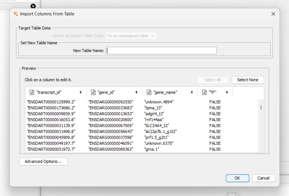
In Cytoscape, go to File > Import >
Table from File
Select the saved text file, click Open, name the table
and select OK
Right-click the column with ids for querying proteins (e.g.,
gene_id) (1), then select Copy Column Values
(2)
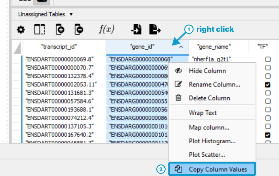
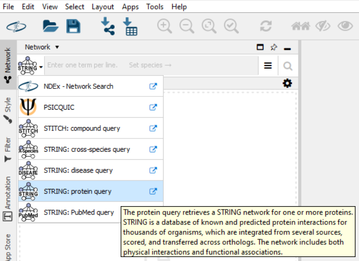
Ensure you are using the Protein Query feature with StringApp.
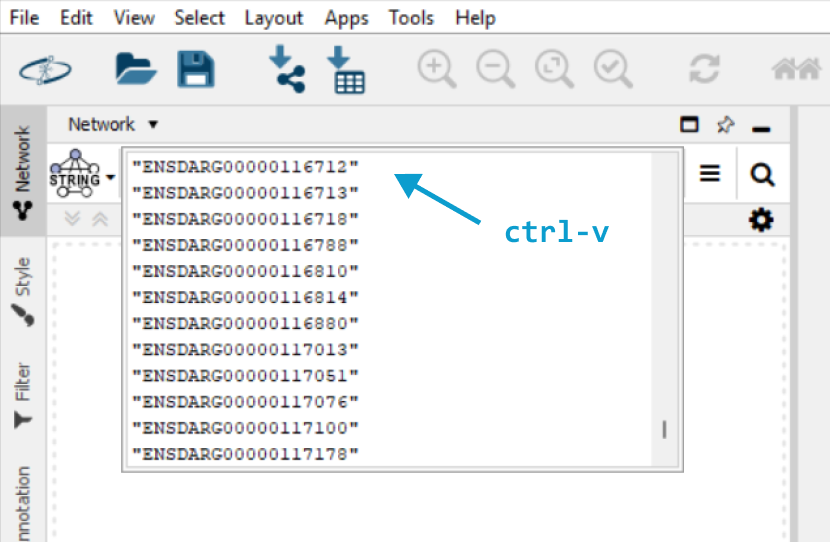
In the StringApp query section, paste
(Ctrl+V) the copied values
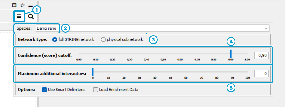
Adjust the query settings:
- Click on the “More options…” icon
- Select the species (e.g., Danio rerio)
- Select the network type2
- Select a confidence score cutoff3
- Make sure that maximum additional interactors is at “0”!4
Visit the STRING documentation to getting a fuller understand of these concepts.
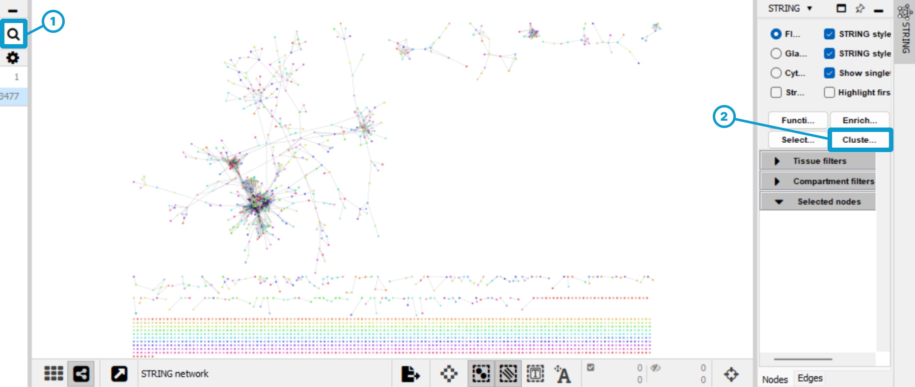
Run the query (1), view the PPI network, then click on “Clustering” (2)
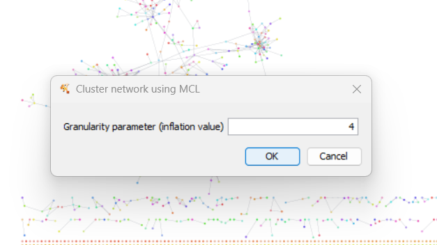
Choose a granularity (inflation) value to adjust cluster sizes5, then click “OK”
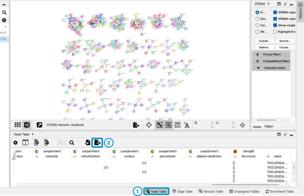
Open the Node Table (1) and click on
the Export Tables to File... icon (2). Finally, save the
table in .csv format within your working directory.
With the node table saved, we can now return to the R environment and import the table.
Using the getclustrs() function,
retrieve and merge the node table with the output of the getregs() function.
Therefor it requires the output from the function used in Step 3, the column name to use for merging and the
nodetable path and filename, as shown below :
dr_t_clustrs <- getclustrs(
  gene_data = dr_t_regs,
  colname_for_merge = "gene_id",
  path = "your/chosen/path",
  nodetable_filename = "filename.csv"
)
For more information on each argument of the function, run
?cluefish::getclustrs().
We can look at the structure of this output:
dplyr::glimpse(dr_t_clustrs)
#> Rows: 775
#> Columns: 5
#> $ gene_id       <chr> "ENSDARG00000000068", "ENSDARG00000000086", "ENSDARG0000…
#> $ transcript_id <chr> "ENSDART00000000069.8", "ENSDART00000132378.4", "ENSDART…
#> $ gene_name     <chr> "nherf1a_g2t1", "itsn1", "pms1_t2", "asnsd1_t2", "unknow…
#> $ TF            <lgl> FALSE, FALSE, TRUE, FALSE, FALSE, FALSE, FALSE, FALSE, F…
#> $ clustr        <int> 139, 140, 27, 172, 159, 56, 47, 36, 187, 164, 144, 52, 6…
We can also get an idea of the size of the clusters:
table(dr_t_clustrs$clustr)
#>
#>   1   2   3   4   5   6   7   8   9  10  11  12  13  14  15  16  17  18  19  20
#>  41  35  22  18  17  14  12  12   8   8   7   7   7   8   6   6   6   6   7   6
#>  21  22  23  24  25  26  27  28  29  30  31  32  33  34  35  36  37  38  39  40
#>   6   6   5   5   6   5   5   5   7   5   5   5   5   5   5   5   5   5   4   4
#>  41  42  43  44  45  46  47  48  49  50  51  52  53  54  55  56  57  58  59  60
#>   5   5   4   4   4   4   4   4   5   4   4   4   4   3   3   4   3   3   3   3
#>  61  62  63  64  65  66  67  68  69  70  71  72  73  74  75  76  77  78  79  80
#>   3   3   3   3   3   5   3   3   3   3   3   3   3   3   3   3   3   3   3   3
#>  81  82  83  84  85  86  87  88  89  90  91  92  93  94  95  96  97  98  99 100
#>   3   3   3   3   3   3   3   3   3   3   3   3   3   3   3   3   3   3   3   3
#> 101 102 103 104 105 106 107 108 109 110 111 112 113 114 115 116 117 118 119 120
#>   3   3   2   2   3   3   2   2   3   2   4   2   2   2   2   2   2   2   2   2
#> 121 122 123 124 125 126 127 128 129 130 131 132 133 134 135 136 137 138 139 140
#>   2   2   2   2   2   2   2   2   2   2   2   2   2   2   2   2   2   2   2   3
#> 141 142 143 144 145 146 147 148 149 150 151 152 153 154 155 156 157 158 159 160
#>   2   2   2   2   2   2   2   2   2   2   2   2   2   2   2   2   2   2   2   2
#> 161 162 163 164 165 166 167 168 169 170 171 172 173 174 175 176 177 178 179 180
#>   2   2   2   2   2   2   2   2   2   2   2   2   2   2   2   2   2   2   2   2
#> 181 182 183 184 185 186 187 188 189 190 191 192 193 194 195 196 197 198 199 200
#>   2   2   2   3   2   2   2   2   2   2   3   2   2   2   3   2   3   2   2   2
#> 201 202 203 204
#>   2   2   2   2
Step 6: Filter clusters
In this step, we filter clusters based on their gene set sizes using the lower cluster size filter. This filter retains only clusters meeting or exceeding a specified minimum size, helping to focus on clusters that are likely biologically relevant.
The function clustrfiltr() applies this
filter, requiring two main arguments:
-
getclustrs_data: the output from thegetclustrs()function - the desired lower cluster size filter value.
Choosing an appropriate lower cluster size limit
The choice of size limit depends on factors such as the type of study, the organism, and prior steps in the PPI network creation and clustering. Setting a higher size limit will retain fewer, larger clusters, while a lower limit will include both large and small clusters. Note that:
- Large clusters may lack specific biological context due to their broad inclusivity.
- Small clusters may suffer from limited statistical support and might not represent distinct biological complexes. Instead, they could reflect case-specific or transient interactions.
Consider these factors when deciding on an appropriate size limit.
dr_t_clustrs_filtr <- clustrfiltr(
  getclustrs_data = dr_t_clustrs,
  size_filtr = 4 # default value
)
For more information on each argument of the function, run
?cluefish::clustrfiltr().
The function outputs a named list with three components:
-
kept: A dataframe of type t holding clusters retained after filtering -
removed: A dataframe of type t holding clusters filtered out -
params: A list of the main parameters used; in this case the choice forsize_filtr
We can take a look at the output’s structure:
dplyr::glimpse(dr_t_clustrs_filtr)
#> List of 3
#>  $ kept   :'data.frame': 411 obs. of  5 variables:
#>   ..$ gene_id      : chr [1:411] "ENSDARG00000003564" "ENSDARG00000003599" "ENSDARG00000005791" "ENSDARG00000006413" ...
#>   ..$ transcript_id: chr [1:411] "ENSDART00000018515.5" "ENSDART00000011251.10" "ENSDART00000175435.2" "ENSDART00000021069.8" ...
#>   ..$ gene_name    : chr [1:411] "dohh" "rpl3_t2" "rpl28_t2" "rpl38" ...
#>   ..$ TF           : logi [1:411] FALSE FALSE FALSE FALSE FALSE FALSE ...
#>   ..$ clustr       : int [1:411] 1 1 1 1 1 1 1 1 1 1 ...
#>  $ removed:'data.frame': 364 obs. of  5 variables:
#>   ..$ gene_id      : chr [1:364] "ENSDARG00000023152" "ENSDARG00000041155" "ENSDARG00000101216" "ENSDARG00000077822" ...
#>   ..$ transcript_id: chr [1:364] "ENSDART00000030984.4" "ENSDART00000139441.2" "ENSDART00000172204.2" "ENSDART00000113752.3" ...
#>   ..$ gene_name    : chr [1:364] "wdr73_g2t1" "morf4l1" "meaf6_t2" "si:dkey-6i22.5" ...
#>   ..$ TF           : logi [1:364] FALSE TRUE TRUE FALSE FALSE FALSE ...
#>   ..$ clustr       : int [1:364] 54 54 54 55 55 55 56 56 56 56 ...
#>  $ params :List of 1
#>   ..$ size_filtr: num 4
#>  - attr(*, "class")= chr "clustrfiltres"
We can also see which clusters were retained:
table(dr_t_clustrs_filtr$kept$clustr)
#>
#>  1  2  3  4  5  6  7  8  9 10 11 12 13 14 15 16 17 18 19 20 21 22 23 24 25 26
#> 41 35 22 18 17 14 12 12  8  8  7  7  7  8  6  6  6  6  7  6  6  6  5  5  6  5
#> 27 28 29 30 31 32 33 34 35 36 37 38 39 40 41 42 43 44 45 46 47 48 49 50 51 52
#>  5  5  7  5  5  5  5  5  5  5  5  5  4  4  5  5  4  4  4  4  4  4  5  4  4  4
#> 53
#>  4
Genes that are not retained in this step have now become lonely genes.
Step 7: Perform cluster-wise functional enrichment
This step applies Over-Representation Analysis (ORA) to characterise
each cluster using the gprofiler2 R package (Kolberg et al. 2020), which interfaces with
g:Profiler’s (Kolberg et al. 2023)
ressources and functions. The g:GOst function performs ORA across
multiple gene lists, analysing against sources such as GO, KEGG, and WP.
For more information on g:Profiler and g:GOst, visit the web interface
here.
The clustrenrich() function,
built on g:GOst, performs cluster-wise ORA.
The function applies g:GOst’s highlighting GO driver terms by considering the underlying topology of annotations, as described in Kolberg et al. 2023.
Consider the following g:GOst key options:
-
sources: Functional data sources to analyse against (e.g. “GO”, “KEGG”) -
domain_scope: Background choice (e.g. “annotated”, “known”, “custom”) -
correction_method: Multiple testing correction method, e.g., FDR -
user_threshold: P-value threshold for significance, e.g. 0.05
These are a few key options, but many others are available. Some
require careful thought to select the best value, method, or scope. For
more details, check the documentation on their site or reading the help
of the function by running ?gprofiler2::gost() in R.
Additionally, two new filters have been integrated with the
construction of the clustrenrich()
function:
-
Biological function size filter (
min_term_sizeandmax_term_size): Filter based on upper and lower gene set size limits to control for biological function specificity
Very large gene sets, which are dependent on the organism, are often associated with broad biological processes. These can introduce noise and obscure more specific functions. Conversely, very small gene sets can be overly specific and may not capture the full biological context of a pathway.
-
Enrichment gene count filter (
ngenes_enrich_filtr): Filters based on the number of genes contributing to enrichment of a cluster.
Small clusters can lead to a higher rate of false positives, and enrichments based on very few genes may not provide substantial biological insight into the cluster itself.
The function data inputs include:
-
clustrfiltr_data: The named list output from theclustrfiltr()function -
dr_genes: The character vector of deregulated genes that can correspond to thegene_idcolumn in the output of thegetids()orgetregs()function. -
bg_genes: The character vector of background genes (preferably from the experiment) that typically corresponds to the ‘gene_id’ column in the output of thegetids()function.
clustr_enrichres <- clustrenrich(
  clustrfiltr_data = dr_t_clustrs_filtr,
  dr_genes = dr_t_regs$gene_id,
  bg_genes = bg_t_ids$gene_id,
  bg_type = "custom_annotated",
  sources = c("GO:BP", "KEGG", "WP"),
  organism = "drerio",
  user_threshold = 0.05,
  correction_method = "fdr",
  exclude_iea = FALSE,
  min_term_size = 5,
  max_term_size = 500,
  only_highlighted_GO = TRUE,
  ngenes_enrich_filtr = 3,
  path = "your/chosen/path",
  output_filename = "filename.rds",
  overwrite = FALSE
)
For more information on each argument of the function, run
?cluefish::clustrenrich().
The output is a named list with four components:
-
dr_g_a_enrich: A dataframe of type g_a holding the cluster-wise enrichment results -
gostres: A named list corresponding to the original result output of g:GOst -
dr_g_a_whole: A dataframe of type g_a holding all the biological function annotations found in the g:profiler database for all the deregulated genes. -
c_simplify_log: A dataframe of tracing the number of biological functions enriched per cluster before and after each filtering step for each source. -
params: A list of the main parameters used; in this case the choice formonoterm_fusion
We can take a look at the structure of the
dr_g_a_enrich dataframe:
#> Rows: 754
#> Columns: 5
#> $ gene_id   <chr> "ENSDARG00000051783", "ENSDARG00000009285", "ENSDARG00000020…
#> $ clustr    <dbl> 1, 1, 1, 1, 1, 1, 1, 1, 1, 1, 1, 1, 1, 1, 1, 1, 1, 1, 1, 1, …
#> $ term_name <chr> "Cytoplasmic ribosomal proteins", "Cytoplasmic ribosomal pro…
#> $ term_id   <chr> "WP:WP324", "WP:WP324", "WP:WP324", "WP:WP324", "WP:WP324", …
#> $ source    <chr> "WP", "WP", "WP", "WP", "WP", "WP", "WP", "WP", "WP", "WP", …
After running the function, we recommend checking if the filters need adjustment, as finding the right lower and upper limits for gene set sizes can be quite a challenge. These limits depend on the organism, the type of transcriptomic data, and what constitutes ‘general’ terms for this study.
To help determine if the size limits are suitable, the following code lists all terms associated with deregulated genes in descending order by size, giving insight into the generality of terms and guiding any needed adjustments:
clustr_enrichres$dr_g_a_whole |>
  dplyr::group_by(term_name) |>
  dplyr::summarise(count = dplyr::n()) |>
  dplyr::arrange(desc(count)) |>
  print(n = 10) # Number of rows to print, adjustable based on the study
#> # A tibble: 3,646 × 2
#>    term_name                           count
#>    <chr>                               <int>
#>  1 biological_process                   1509
#>  2 cellular process                     1299
#>  3 metabolic process                     903
#>  4 organic substance metabolic process   855
#>  5 primary metabolic process             832
#>  6 nitrogen compound metabolic process   776
#>  7 cellular metabolic process            771
#>  8 macromolecule metabolic process       718
#>  9 KEGG root term                        707
#> 10 biological regulation                 556
#> # ℹ 3,636 more rows
If you have the DT package installed, you can view this
data interactively in the viewer pane:
clustr_enrichres$dr_g_a_whole |>
  dplyr::group_by(term_name) |>
  dplyr::summarise(count = dplyr::n()) |>
  DT::datatable(
    options = list(pageLength = 10
    ),
    filter = 'top',
    class = c("compact")
  )
Step 8: Merge clusters
Following cluster characterisation, this step consists in identifying and merging clusters that share the same enriched biological functions from at least one specified data source (e.g. GO, KEGG etc.) in the ORA. This step allows us to merge multiple clusters where the gene proteins were not found to be sufficiently interactive in STRING to be considered a single cluster. However, functional enrichment revealed that they participate in the same biological processes. Therefore, clusters that do merge form a larger and more comprehensive cluster, holding a unique biological context.
To do so, the step uses the clustrfusion() function,
which requires the output of the clustrenrich() function as
its input data.
The merging process is conducted separately
for each data source, in descending order of the total number of unique
genes present in both the data source and the background list. An
optional parameter, monoterm_fusion, can be set to
TRUE to restrict merging to clusters that share a single,
identical enrichment term in at least one source. This ensures that
merged clusters are consistently linked to a specific biological
function, maintaining a coherent biological context. By default this is
set to FALSE as the merging process becomes highly
stringent, as it requires clusters to be associated with the same unique
biological function. This can significantly limit the likelihood of
merging.
clustr_fusionres <- clustrfusion(
  clustrenrich_data = clustr_enrichres,
  monoterm_fusion = FALSE
)
The output is a named list with four components:
-
dr_g_a_fusion: A dataframe of type g_a holding the cluster fusion results -
dr_g_a_fusion: A dataframe of type c_a holding the cluster fusion results -
c_fusionlog: A dataframe tracing cluster fusion events, indicating the sources from which they originated (e.g. GO, KEGG or WP) -
params: A list of the main parameters used; in this case the choice formonoterm_fusion
We can take a look at the structure of the output:
dplyr::glimpse(clustr_fusionres)
#> List of 4
#>  $ dr_g_a_fusion:'data.frame':   754 obs. of  6 variables:
#>   ..$ gene_id   : chr [1:754] "ENSDARG00000051783" "ENSDARG00000009285" "ENSDARG00000020197" "ENSDARG00000043509" ...
#>   ..$ old_clustr: num [1:754] 1 1 1 1 1 1 1 1 1 1 ...
#>   ..$ new_clustr: num [1:754] 1 1 1 1 1 1 1 1 1 1 ...
#>   ..$ term_name : chr [1:754] "Cytoplasmic ribosomal proteins" "Cytoplasmic ribosomal proteins" "Cytoplasmic ribosomal proteins" "Cytoplasmic ribosomal proteins" ...
#>   ..$ term_id   : chr [1:754] "WP:WP324" "WP:WP324" "WP:WP324" "WP:WP324" ...
#>   ..$ source    : chr [1:754] "WP" "WP" "WP" "WP" ...
#>  $ dr_c_a_fusion:'data.frame':   133 obs. of  7 variables:
#>   ..$ old_clustr : num [1:133] 1 1 1 1 1 1 2 2 2 2 ...
#>   ..$ new_clustr : num [1:133] 1 1 1 1 1 1 1 1 1 1 ...
#>   ..$ term_name  : chr [1:133] "Cytoplasmic ribosomal proteins" "embryo development ending in birth or egg hatching" "myeloid cell differentiation" "ribonucleoprotein complex biogenesis" ...
#>   ..$ term_size  : int [1:133] 60 180 89 175 102 351 60 7 102 351 ...
#>   ..$ term_id    : chr [1:133] "WP:WP324" "GO:0009792" "GO:0030099" "GO:0022613" ...
#>   ..$ source     : chr [1:133] "WP" "GO:BP" "GO:BP" "GO:BP" ...
#>   ..$ highlighted: logi [1:133] FALSE TRUE TRUE TRUE FALSE TRUE ...
#>  $ c_fusionlog  :'data.frame':   754 obs. of  4 variables:
#>   ..$ old_clustr        : num [1:754] 1 1 1 1 1 1 1 1 1 1 ...
#>   ..$ after_GO:BP_fusion: num [1:754] 1 1 1 1 1 1 1 1 1 1 ...
#>   ..$ after_KEGG_fusion : num [1:754] 1 1 1 1 1 1 1 1 1 1 ...
#>   ..$ after_WP_fusion   : num [1:754] 1 1 1 1 1 1 1 1 1 1 ...
#>  $ params       :List of 1
#>   ..$ monoterm_fusion: logi FALSE
#>  - attr(*, "class")= chr "clustrfusion"
Step 9: Fish lonely genes
Genes not assigned to any cluster are referred to as lonely genes. These genes are not typically explored because they do not contribute to functional enrichment, and thus, they do not help in characterising the data. This step involves “fishing” these lonely genes into existing clusters.
Genes become lonely in one of two cases :
- they are initially not sufficiently interactive with another protein complex to participate in or form a cluster
- they were initially part of a cluster but failed to pass the cluster size filtering step, thus falling into the lonely cluster.
To “fish” these genes meaningfully, the lonelyfishing() function
matches lonely genes with clusters that share the same functional
annotations, and incorporates them into the cluster.
Each lonely gene has a friendliness metric, representing the number of potentiel clusters it can be incorporated into. The friendliness filter allows the user to set a limit to this metric, solely fishing genes that fall below this limit, while genes that exceed the limit remain in the lonely cluster.
Low values of this limit, such as 1 to 3, result in fewer lonely genes being incorporated but reduce redundancy between clusters. Although this approach does not fish as much, it ensures that lonely genes associated with a wide range of biological functions are not distributed across many clusters, thereby minimising noise in the results. By default, the limit is set to 0, meaning it is not applied, and all lonely genes eligible for fishing are incorporated.
The function’s data inputs include:
-
dr_data: A dataframe of type t that typically corresponds to the output ofgetids()orgetregs(). This input holds at leastgene_idandterm_namecolumns, respectively containing gene identifiers and biological function annotations for the deregulated genes. Recommended to hold alsotranscript_idfor futur functions. -
clustrenrich_data: The namedlistoutput of theclustrenrich()function. -
clustrfusion_data: The namedlistoutput of theclustrfusion()function.
lonely_fishres <- lonelyfishing(
  dr_data = dr_t_regs,
  clustrenrich_data = clustr_enrichres,
  clustrfusion_data = clustr_fusionres,
  friendly_limit = 0,
  path = "your/chosen/path",
  output_filename = "filename.rds",
  overwrite = FALSE
)
For more information on each argument of the function, run
?cluefish::lonelyfishing().
The output of the lonelyfishing() is a named
list holding 3 components, where:
-
dr_g_a_fishing: A dataframe of type t_c_a holding the lonely fishing results -
dr_c_a_fishing: A dataframe of the lonely fishing results similar to theclustrfusion_data$dr_c_a_fusiondataframe with each row being a combination of cluster ID and biological function annotation. -
params: A list of the main parameters used; in this case thefriendly_limit
We can take a look a the structure of the output:
dplyr::glimpse(lonely_fishres)
#> List of 3
#>  $ dr_t_c_a_fishing:'data.frame':    9841 obs. of  10 variables:
#>   ..$ transcript_id: chr [1:9841] "ENSDART00000175435.2" "ENSDART00000175435.2" "ENSDART00000175435.2" "ENSDART00000175435.2" ...
#>   ..$ gene_id      : chr [1:9841] "ENSDARG00000005791" "ENSDARG00000005791" "ENSDARG00000005791" "ENSDARG00000005791" ...
#>   ..$ gene_name    : chr [1:9841] "rpl28_t2" "rpl28_t2" "rpl28_t2" "rpl28_t2" ...
#>   ..$ TF           : logi [1:9841] FALSE FALSE FALSE FALSE FALSE FALSE ...
#>   ..$ old_clustr   : chr [1:9841] "1" "1" "1" "1" ...
#>   ..$ new_clustr   : chr [1:9841] "1" "1" "1" "1" ...
#>   ..$ friendliness : int [1:9841] 1 1 1 1 1 1 1 1 1 1 ...
#>   ..$ term_name    : chr [1:9841] "embryo development ending in birth or egg hatching" "embryo development ending in birth or egg hatching" "embryo development ending in birth or egg hatching" "embryo development ending in birth or egg hatching" ...
#>   ..$ term_id      : chr [1:9841] "GO:0009792" "GO:0009792" "GO:0009792" "GO:0009792" ...
#>   ..$ source       : chr [1:9841] "GO:BP" "GO:BP" "GO:BP" "GO:BP" ...
#>  $ dr_c_a_fishing  :'data.frame':    242 obs. of  7 variables:
#>   ..$ old_clustr : chr [1:242] "1" "1" "1" "1" ...
#>   ..$ new_clustr : chr [1:242] "1" "1" "1" "1" ...
#>   ..$ term_name  : chr [1:242] "Cytoplasmic ribosomal proteins" "embryo development ending in birth or egg hatching" "myeloid cell differentiation" "Protein export" ...
#>   ..$ term_size  : int [1:242] 60 180 89 26 175 102 351 60 7 102 ...
#>   ..$ term_id    : chr [1:242] "WP:WP324" "GO:0009792" "GO:0030099" "KEGG:03060" ...
#>   ..$ source     : chr [1:242] "WP" "GO:BP" "GO:BP" "KEGG" ...
#>   ..$ highlighted: logi [1:242] FALSE TRUE TRUE FALSE TRUE FALSE ...
#>  $ params          :List of 1
#>   ..$ friendly_limit: num 0
#>  - attr(*, "class")= chr "lonelyfishingres"
Step 10: Perform functional enrichment of the lonely cluster genes
The lonely cluster, consisting of the remaining lonely genes, can
undergo a simple functional enrichment analysis to gain further insight
into the biological context it may contain. The customisations used in
the earlier cluster-wise enrichment analysis are fully applicable here
as well. Therefore, the parameters were set to match those chosen in the
previous cluster-wise functional enrichment analysis. The function simplenrich() enables a
single ORA, with parameters mirroring the earlier clustrenrich() function.
The only difference is that a input_genes argument is
created to take the list of genes.
First, we need to extract the lonely genes:
lonelycluster_data <- lonely_fishres$dr_t_c_a_fishing |>
  dplyr::filter(new_clustr == "Lonely")
Then, we can conduct enrichment:
lonely_clustr_analysis_res <- simplenrich(
  input_genes = lonelycluster_data$gene_id,
  bg_genes = bg_t_ids$gene_id,
  bg_type = "custom_annotated",
  sources = c("GO:BP", "KEGG", "WP"),
  organism = "drerio",
  user_threshold = 0.05,
  correction_method = "fdr",
  only_highlighted_GO = TRUE,
  min_term_size = 5,
  max_term_size = 500,
  ngenes_enrich_filtr = 3,
  path = "your/chosen/path",
  output_filename = "filename.rds",
  overwrite = FALSE
)
For more information on each argument of the function, run
?cluefish::simplenrich().
The output is a named list with two components:
-
unfiltered: A named list of the unfiltered enrichment results, holding two sub-components :-
dr_g_a: A dataframe of type g_a holding the simple enrichment results -
gostres: A named list of the original result output of g:GOst
-
-
filtered: A named list of the filtered enrichment results, holding three sub-components:-
dr_g_a: A dataframe of type g_a holding the simple enrichment results -
dr_a: A dataframe of type a holding the simple enrichment -
params: A list of the main parameters used
-
We can take a look at the filtered results, with each row corresponding to an enriched term :
dplyr::glimpse(lonely_clustr_analysis_res$filtered$dr_a)
#> Rows: 12
#> Columns: 17
#> $ query                 <chr> "query_1", "query_1", "query_1", "query_1", "que…
#> $ significant           <lgl> TRUE, TRUE, TRUE, TRUE, TRUE, TRUE, TRUE, TRUE, …
#> $ p_value               <dbl> 2.09e-13, 1.12e-06, 1.06e-02, 1.26e-02, 2.98e-02…
#> $ term_size             <int> 70, 139, 41, 106, 15, 23, 268, 143, 72, 46, 78, …
#> $ query_size            <int> 763, 763, 763, 763, 763, 763, 177, 177, 177, 177…
#> $ intersection_size     <int> 26, 26, 9, 15, 5, 6, 22, 14, 9, 6, 10, 6
#> $ precision             <dbl> 0.03408, 0.03408, 0.01180, 0.01966, 0.00655, 0.0…
#> $ recall                <dbl> 0.3714, 0.1871, 0.2195, 0.1415, 0.3333, 0.2609, …
#> $ term_id               <chr> "GO:0002088", "GO:0007601", "GO:0000041", "GO:00…
#> $ source                <chr> "GO:BP", "GO:BP", "GO:BP", "GO:BP", "GO:BP", "GO…
#> $ term_name             <chr> "lens development in camera-type eye", "visual p…
#> $ effective_domain_size <int> 15468, 15468, 15468, 15468, 15468, 15468, 5714, …
#> $ source_order          <int> 681, 3094, 17, 13905, 1212, 13702, 280, 279, 220…
#> $ parents               <list> <"GO:0043010", "GO:0048856">, "GO:0050953", "GO:…
#> $ evidence_codes        <chr> "IMP IGI,IBA,IBA,IBA,IBA,IBA,IBA,IBA,IBA,IBA,IB…
#> $ intersection          <chr> "ENSDARG00000013963,ENSDARG00000016793,ENSDARG00…
#> $ highlighted           <lgl> TRUE, TRUE, TRUE, TRUE, TRUE, TRUE, FALSE, FALSE…
Outputs to explore the results
Homemade functions
To fully explore the Cluefish results, including DR modelling metrics
from DRomics outputs is required.
-
The
results_to_csv()function generates a summary .csv file from the Cluefish workflow results, supporting manual exploration.It requires two main data inputs:
-
lonelyfishing_data: The named list output of thelonelyfishing()function. -
bmdboot_data: The DRomics bmdboot dataframe results afterDRomics::bmdboot()or following the additional stepDRomics::bmdfilter(). This data should include the deregulated transcript identifiers from Step 2.
results_to_csv(
 lonelyfishing_data = lonely_fishres,
 bmdboot_data = b_definedCI,
 path = "your/chosen/path",
 output_filename = "filename.csv",
 overwrite = TRUE
)
For more information on each argument of the function, run
?cluefish::results_to_csv(). -
Cluefish also leverages DRomics visualisation functions,
like DRomics::curvesplot(), to plot fitted dose-response
curves.
-
The
curves_to_pdf()function generates a .pdf of the fitted curves for each cluster’s gene set, offering visual insight into cluster composition.It requires five main inputs:
-
lonelyfishing_data: The named list output of thelonelyfishing()function. -
bmdboot_data: TheDRomicsbmdbootdataframe results afterDRomics::bmdboot()or following the additional stepDRomics::bmdfilter(). This must correspond to the data loaded containing the deregulated transcript identifiers in the Step 2. -
clustrfusion_data: The named list output of theclustrfusion()function. -
tested_doses: A vector of the tested doses that can be found in the output of theDRomics::drcfit()function asunique(f$omicdata$dose). -
annot_order: A vector specifying the prioritised order of annotation sources used in theclustrenrich()function.
The
annot_orderspecifies the preferred order of annotation sources for assigning a primary descriptor to each cluster. If an enriched function is found in the first source listed, that function will be used as the primary descriptor for the cluster. This order allows you to prioritise annotation databases based on their relevance and the quality of information they provide for your study.
curves_to_pdf(
 lonelyfishing_data = lonely_fishres,
 bmdboot_data = b_definedCI,
 clustrfusion_data = clustr_fusionres,
 tested_doses = unique(f$omicdata$dose),
 annot_order = c("GO:BP", "KEGG", "WP"),
 colorby = "trend",
 addBMD = TRUE,
 scaling = TRUE,
 npoints= 100,
 free.y.scales = FALSE,
 xmin = 0.1,
 xmax = 100,
 dose_log_transfo = TRUE,
 line.size = 0.7,
 line.alpha = 0.4,
 point.size = 2,
 point.alpha = 0.4,
 xunit = "µg/L",
 xtitle = "Dose (µg/L)",
 ytitle = "Signal",
 colors = c("inc" = "#1B9E77", "dec" = "#D95F02", "U" = "#7570B3", "bell" = "#E7298A"),
 path = paste0("outputs/", file_date, "/"),
 output_filename = paste0("workflow_curvesplots_", file_date, ".pdf"),
 overwrite = TRUE
)
For more information on each argument of this function, run
?cluefish::curves_to_pdf(). For more information on each argument of theDRomics::curvesplot(), run?DRomics::curvesplot(). -
Quarto report templates
The Cluefish compendium includes Quarto report templates that can streamline the summarisation of Cluefish results, enhancing interpretability and ease of use. These reports are auto-generated but can be customised as needed.
The available templates include:
report_workflow_results.qmdThis report summarises key findings from the DRomics analysis and workflow results. It includes visual summaries like BMD plots per cluster and interactive visualisations using theplotlyR package, helping to prioritise results and explore each cluster.report_lonely_results.qmdThis report focuses on the Lonely cluster, summarising the results of genes that did not associate with other clusters. It includesplotlyinteractiveDRomicsplots like BMD distributions, trend-colored fitted curves, and ECDF plots for detailed exploration.report_comparison_resultsThis report compares Cluefish with a standard workflow (simplenrich()). A script is available to perform the standard approach script can be found in theanalysesfolder, under the name:standard-pipeline.
To generate these reports, use the custom render_qmd()
function, which builds on quarto::quarto_render() and
allows output to a designated directory. It supports all
quarto::quarto_render() arguments.
Important: Some adaptations may be needed for directory paths, file naming, or other settings.
License
The Cluefish project code is distributed under the CECILL v2.1 license. Illustrations are licensed under CC-BY-SA-4.0 license.
Session info
#> R version 4.5.1 (2025-06-13)
#> Platform: x86_64-pc-linux-gnu
#> Running under: Ubuntu 24.04.3 LTS
#>
#> Matrix products: default
#> BLAS:   /usr/lib/x86_64-linux-gnu/openblas-pthread/libblas.so.3
#> LAPACK: /usr/lib/x86_64-linux-gnu/openblas-pthread/libopenblasp-r0.3.26.so;  LAPACK version 3.12.0
#>
#> locale:
#>  [1] LC_CTYPE=fr_FR.UTF-8       LC_NUMERIC=C
#>  [3] LC_TIME=fr_FR.UTF-8        LC_COLLATE=fr_FR.UTF-8
#>  [5] LC_MONETARY=fr_FR.UTF-8    LC_MESSAGES=fr_FR.UTF-8
#>  [7] LC_PAPER=fr_FR.UTF-8       LC_NAME=C
#>  [9] LC_ADDRESS=C               LC_TELEPHONE=C
#> [11] LC_MEASUREMENT=fr_FR.UTF-8 LC_IDENTIFICATION=C
#>
#> time zone: Europe/Paris
#> tzcode source: system (glibc)
#>
#> attached base packages:
#> [1] stats     graphics  grDevices datasets  utils     methods   base
#>
#> other attached packages:
#> [1] cluefish_1.0.1 ggplot2_3.5.2
#>
#> loaded via a namespace (and not attached):
#>   [1] RColorBrewer_1.1-3          rstudioapi_0.17.1
#>   [3] jsonlite_2.0.0              magrittr_2.0.3
#>   [5] farver_2.1.2                rmarkdown_2.29
#>   [7] fs_1.6.6                    ragg_1.4.0
#>   [9] vctrs_0.6.5                 memoise_2.0.1
#>  [11] htmltools_0.5.8.1           S4Arrays_1.4.1
#>  [13] usethis_3.1.0               progress_1.2.3
#>  [15] curl_7.0.0                  SparseArray_1.4.8
#>  [17] sass_0.4.10                 bslib_0.9.0
#>  [19] htmlwidgets_1.6.4           quarto_1.5.0
#>  [21] desc_1.4.3                  httr2_1.2.1
#>  [23] plotly_4.11.0               cachem_1.1.0
#>  [25] mime_0.13                   lifecycle_1.0.4
#>  [27] DRomics_2.6-2               pkgconfig_2.0.3
#>  [29] Matrix_1.7-3                R6_2.6.1
#>  [31] fastmap_1.2.0               GenomeInfoDbData_1.2.14
#>  [33] MatrixGenerics_1.16.0       shiny_1.11.1
#>  [35] digest_0.6.37               ps_1.9.1
#>  [37] AnnotationDbi_1.70.0        S4Vectors_0.46.0
#>  [39] DESeq2_1.44.0               rprojroot_2.1.0
#>  [41] pkgload_1.4.0               crosstalk_1.2.1
#>  [43] textshaping_1.0.1           GenomicRanges_1.56.2
#>  [45] RSQLite_2.4.2               filelock_1.0.3
#>  [47] httr_1.4.7                  abind_1.4-8
#>  [49] compiler_4.5.1              here_1.0.1
#>  [51] remotes_2.5.0               bit64_4.6.0-1
#>  [53] withr_3.0.2                 BiocParallel_1.38.0
#>  [55] DBI_1.2.3                   pkgbuild_1.4.8
#>  [57] biomaRt_2.60.1              rappdirs_0.3.3
#>  [59] DelayedArray_0.30.1         sessioninfo_1.2.3
#>  [61] tools_4.5.1                 httpuv_1.6.16
#>  [63] glue_1.8.0                  promises_1.3.3
#>  [65] grid_4.5.1                  generics_0.1.4
#>  [67] gtable_0.3.6                tidyr_1.3.1
#>  [69] data.table_1.17.8           hms_1.1.3
#>  [71] utf8_1.2.6                  xml2_1.3.8
#>  [73] XVector_0.48.0              BiocGenerics_0.54.0
#>  [75] pillar_1.11.0               stringr_1.5.1
#>  [77] limma_3.64.3                later_1.4.2
#>  [79] dplyr_1.1.4                 BiocFileCache_2.12.0
#>  [81] lattice_0.22-7              renv_1.1.5
#>  [83] bit_4.6.0                   tidyselect_1.2.1
#>  [85] locfit_1.5-9.12             Biostrings_2.76.0
#>  [87] miniUI_0.1.2                knitr_1.50
#>  [89] gridExtra_2.3               IRanges_2.42.0
#>  [91] SummarizedExperiment_1.34.0 stats4_4.5.1
#>  [93] xfun_0.53                   Biobase_2.68.0
#>  [95] statmod_1.5.0               devtools_2.4.5
#>  [97] matrixStats_1.5.0           DT_0.33
#>  [99] stringi_1.8.7               UCSC.utils_1.4.0
#> [101] lazyeval_0.2.2              yaml_2.3.10
#> [103] evaluate_1.0.4              codetools_0.2-20
#> [105] tibble_3.3.0                BiocManager_1.30.26
#> [107] cli_3.6.5                   xtable_1.8-4
#> [109] systemfonts_1.2.3           processx_3.8.6
#> [111] jquerylib_0.1.4             Rcpp_1.1.0
#> [113] GenomeInfoDb_1.44.1         dbplyr_2.5.0
#> [115] gprofiler2_0.2.3            png_0.1-8
#> [117] parallel_4.5.1              ggfortify_0.4.19
#> [119] ellipsis_0.3.2              pkgdown_2.1.3
#> [121] blob_1.2.4                  prettyunits_1.2.0
#> [123] profvis_0.4.0               urlchecker_1.0.1
#> [125] viridisLite_0.4.2           scales_1.4.0
#> [127] purrr_1.1.0                 crayon_1.5.3
#> [129] rlang_1.1.6                 KEGGREST_1.44.1